Power BI: Fun with DAX

Power BI's secret sauce is DAX (Data Analysis Expressions) – a formula language that lets you create dynamic calculations and advanced analytics in your reports. If you’ve ever used Excel formulas, DAX will feel familiar (think of it as Excel formulas on steroids!), but it’s built for Power BI’s relational data model and interactive visuals. In short, DAX empowers Power BI users to turn raw data into meaningful insights with custom calculations that go far beyond out-of-the-box measures. According to Microsoft, “DAX is a collection of functions, operators, and constants that can be used in a formula or expression to calculate and return one or more values”. Using DAX, you can create new information from data already in your model – for example, analyzing growth percentage across product categories, or calculating year-over-year trends that basic visuals alone can’t show. Over 200 DAX functions cover everything from simple sums and averages to complex filtering and time intelligence calculations. In this blog post, we’ll dive into DAX syntax, explore many useful DAX functions (with plenty of examples!), and share tips for writing efficient DAX. The tone is educational but casual – so grab a coffee, and let’s have fun with DAX!

DAX Syntax and Structure in a Nutshell

Before jumping into specific functions, let’s get familiar with DAX syntax and how to write DAX in Power BI. DAX formulas always start with an equals sign (=) and are typically written for measures or calculated columns in your data model. A measure is a dynamic calculation (like Total Sales or YOY Growth) that evaluates based on report context (filters, slicers, etc.). At the same time, a calculated column computes a value for each row of a table (and is stored in the model). Most of our discussion will focus on measures, since they’re the go-to for most analytics.

Basic DAX formula structure: MeasureName = <DAX expression>. For example, a simple measure might be:

Total Sales = SUM(Sales[SalesAmount])

This measure, Total Sales, sums up the SalesAmount column in the Sales table. The syntax elements include the measure name (Total Sales), the equals sign, and a DAX function (SUM) with its arguments in parentheses (here, we pass the Sales[SalesAmount] column as the argument). DAX uses fully qualified column references (TableName[ColumnName]), as seen with Sales[SalesAmount].

Context is key: Unlike Excel, where formulas usually calculate on a fixed cell range, DAX measures are evaluated in different filter contexts depending on your report. For instance, if you put Total Sales in a chart by Country, the measure will compute the sum of SalesAmount for each Country. If you filter the report to a particular year, the measure respects that filter automatically. This dynamic behaviour makes DAX (and Power BI) so powerful.

 Creating a new measure in Power BI

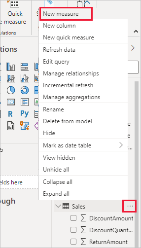
You can add a measure by right-clicking a table in the Fields list (or using the Home > New Measure button). Give the measure a name and write your DAX formula in the formula bar that appears. In the example above, we created Total Sales by writing Total Sales = SUM(Sales[SalesAmount]). Once created, the measure appears in the Fields pane (with a calculator icon ∑) under your chosen table.

The DAX formula bar in Power BI Desktop

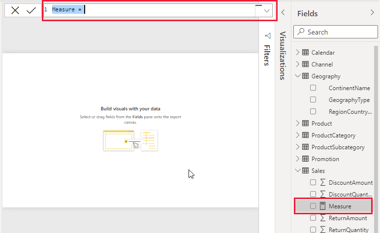
When you create or edit a measure, the formula bar (highlighted in red) lets you enter DAX. You can use IntelliSense (autocomplete) to help find functions and columns as you type. Start with your measure name and equals sign in the formula bar, then build the expression. You can even format the code with line breaks for readability (press Alt+Enter for a new line in the formula bar). Writing DAX feels similar to writing a formula in Excel, but remember that DAX is case-insensitive for function names (e.g. SUM or Sum works the same) and you refer to tables/columns by name. Once you hit the checkmark or press Enter, Power BI validates the formula. If there’s a syntax error (like a missing parenthesis), you’ll get an error prompt to fix it.

Now that we have the basics covered, let’s explore some of the most useful DAX functions and see how they can level up your Power BI analysis!

Essential DAX Functions and Examples

DAX has a rich library of functions. We’ll highlight some of the most commonly used and powerful ones for intermediate/advanced users. Each function solves a different problem – from controlling filter context, iterating over tables, and performing conditional logic. For each function, we’ll explain what it does and give an example formula.

• CALCULATE – The Filter Context Magician

If DAX had a king, it would be CALCULATE. The CALCULATE function evaluates an expression in a modified filter context. In plain English, CALCULATE can take an existing measure or expression and apply filters to it (or override filters) to compute something under specific conditions. It’s incredibly powerful for defining measures like “sales for a specific region” or “sales excluding a certain product”.

What it does: CALCULATE accepts at least two parameters: CALCULATE(<Expression>, <Filter1>, <Filter2>, ...). The first is the expression (often a sum or other measure), and subsequent arguments are filters to apply. These filters can be written as criteria (e.g. Table[Column] = value), or using filter functions like FILTER, ALL, etc. CALCULATE then returns the result of the expression as if those filter conditions were in place.

Example: Suppose we want a measure for Blue Product Sales that totals sales only for products whose color is "Blue". We can write:

Blue Sales = CALCULATE( SUM(Sales[SalesAmount]), 'Product'[Color] = "Blue" )

Here, SUM(Sales[SalesAmount]) is the expression, and 'Product'[Color] = "Blue" is a filter condition. This measure will ignore all sales except those where the Product color is Blue. You could use Blue Sales in a visual, which will always show the sales of blue products, regardless of other filters on Product colour. In effect, CALCULATE changed the filter context to include only blue products for that calculation. As Microsoft’s documentation explains, CALCULATE adds or overrides filters – if the report already had a filter on Product Color, CALCULATE’s filter would replace it for this measure.

Another superpower of CALCULATE is that it performs context transition: when used in a row context (like inside a calculated column or iterator), it can automatically turn the current row into a filter context. This is an advanced concept, but CALCULATE is the only function that can alter filters this way, which is why it’s used in many DAX patterns.

In summary, CALCULATE is your go-to for defining measures with special filter conditions or calculations that differ from the everyday context. You’ll see CALCULATE combined with many other functions (including several below).

• FILTER – Slicing Tables the Dynamic Way

The FILTER function in DAX allows you to retrieve a subset of rows from a table. FILTER is a table function (meaning it returns a table of results, not a single value). Its syntax is FILTER(<Table>, <Condition>). The result is a table with only the rows from <Table> that meet the given <Condition> (which is a boolean test expression).

When to use FILTER: FILTER is often used inside other functions requiring a table input. A typical pattern uses FILTER within CALCULATE to apply more complex filters than simple equality. For example, you can filter a Sales table to “only include transactions above $1000” and then sum them.

Example: Let’s say we want to calculate High Value Sales (sales where each transaction is over $1000). We could do:

High Value Sales = CALCULATE( SUM(Sales[SalesAmount]), FILTER( Sales, Sales[SalesAmount] > 1000 ) )

Here, FILTER(Sales, Sales[SalesAmount] > 1000) yields a filtered table of only those sales records with amount > 1000. CALCULATE then sums the SalesAmount over that filtered table. This pattern (CALCULATE + FILTER) is potent for applying arbitrary conditions.

A key thing to note: FILTER creates a row context while iterating the table, but it’s generally not as optimized as using simple filter arguments in CALCULATE. If your filter condition is simple (like a single column equals a value or IN a list), using it directly in CALCULATE might be faster. But for conditions involving measures or more complex logic, FILTER is the way to go.

One more example without CALCULATE: You can also use FILTER to create a calculated table. For instance, a new calculated table of VIP Customers could be defined as VIP Customers = FILTER(Customers, Customers[TotalSales] > 100000). That would produce a table of customers with sales over 100k (assuming TotalSales is somehow computed per customer).

Remember that FILTER (and other table functions) must be embedded in a context that expects a table – you can’t just drop FILTER alone in a report. That’s why you often see it inside CALCULATE or inside iterators like SUMX. Also, multiple conditions in FILTER can be combined using && (AND) or || (OR), as in FILTER(Sales, Sales[Region]="North" && Sales[Year]=2023).

• SUMX (and the X-Family) – Row-by-Row Iteration

Next up are the X functions, such as SUMX, AVERAGEX, MAXX, MINX, etc. The X indicates these functions perform an iteration over a table, evaluating an expression for each row and then aggregating the results. SUMX is the most famous of the bunch, and it is used to sum up an expression over a table.

What SUMX does: SUMX(<Table>, <Expression>) goes row by row through the <Table>, evaluates the <Expression> for each row, and then returns the sum of all those expression values. It’s a for-loop + sum in one function.

When to use it: Use SUMX to sum something that can’t be expressed as a simple column reference. For example, summing a calculated value like Price * Quantity for each row, or Revenue - Cost per row. The regular SUM() (without X) is more efficient if you need a plain column sum. SUMX is for those cases where a direct SUM won’t do.

Example: Suppose our sales table has separate columns for UnitPrice and Quantity, and we want a measure of Total Sales Revenue (UnitPrice * Quantity summed up). We can write:

Total Revenue = SUMX( Sales, Sales[UnitPrice] * Sales[Quantity] )

This will multiply UnitPrice by Quantity on each row of the Sales table and add all those up to get total revenue. If we tried to do this with just SUM, we’d have to create a calculated column first (UnitPrice * Quantity) and then sum it—SUMX allows us to do it on the fly without a stored column.

Another example: Average Price could be AVERAGEX( Sales, Sales[UnitPrice] ) which effectively averages the UnitPrice across all sales (taking into account the current filter context for Sales rows).

Remember that iterators like SUMX can be slower on large tables than equivalent built-in aggregations. Always prefer a non-X function if it can achieve the same result. For instance, SUM(Sales[SalesAmount]) is faster than SUMX(Sales, Sales[SalesAmount]) because the engine can optimize the direct column sum. Use X functions when you need that per-row calculation logic.

• ALL – Ignoring Filters (for Grand Totals and More)

The ALL function is a filter modifier that returns all table rows or column values, ignoring any filters that might be applied. In other words, ALL lets you remove filters. CALCULATE often uses it to override the current filter context on specific columns or tables.

Usage: ALL(Table) returns all rows of the specified table, and ALL(Table[Column]) returns all values of that column, ignoring any filters on that column. There are also related functions like ALLSELECTED (which considers only filters from outside the visual, ignoring those within the visual) and ALLEXCEPT (which removes all filters except those specified).

When to use ALL: A common scenario is calculating percentages of a total. For example, if you want to compute “% of total sales,” you might need the numerator to be the sales for the current context (e.g., the current region or product) and the denominator to be the sales for all contexts (total sales overall). ALL helps with the denominator by clearing filters. Another use is creating measures that consistently show a constant value regardless of filters (like a target or a total benchmark).

Example: % of Total Sales measure:

Total Sales = SUM(Sales[SalesAmount]) -- base measure % of Total Sales = DIVIDE( [Total Sales], CALCULATE([Total Sales], ALL(Sales)) )

Here, CALCULATE([Total Sales], ALL(Sales)) computes total sales with all filters removed from the Sales table – effectively the grand total sales. The DIVIDE then gives us the current context sales divided by the overall sales. The result is a percentage that shows, say, each product’s contribution to total sales. If a report is filtered to a region, the numerator is that region’s sales, while the denominator (thanks to ALL) still computes using all areas.

Another example: Ignoring a specific filter. If you have a measure that should ignore only the Product Category filter but respect others, you could use ALL(Product[Category]) inside CALCULATE. For instance, Category Ignored Sales = CALCULATE( [Total Sales], ALL(Product[Category]) ). This removes any slicer or filter on Category while calculating Total Sales, but still respects filters on other dimensions like Region or Date.

In summary, ALL is your friend when you need to break out of the current filter context. Just use it carefully – if you remove too many filters, you might inadvertently calculate something unintended. Usually, you’ll pair ALL with specific columns or tables that make sense for your calc.

• RELATED – Lookup Values from Related Tables

The RELATED function is used in DAX to fetch a value from another table related to the current table. It works in row context (like calculated columns or iterators) to perform a lookup based on existing relationships in your data model. If you’re familiar with VLOOKUP in Excel or LOOKUPVALUE in DAX (which is similar), RELATED is the simple way to grab a value from a lookup table.

When to use RELATED: You’ll most often use RELATED in a calculated column. For example, suppose you have a sales table related to a product table, and you want a calculated column in the sales for product category. In that case, you can use RELATED to pull the category from the Product table into each sales row. RELATED works when there is a one-to-many relationship (or one-to-one) and you are on the “many” side trying to get data from the “one” side. It won’t work in the opposite direction (for that, you’d use RELATEDTABLE or other techniques).

Example: Imagine a Product lookup table (one row per product, with columns like ProductName, Category, Price) and an OrderDetails table (many rows, each with a ProductID). In OrderDetails, if we want a column for the Category of each product sold, we could write:

Category = RELATED(Product[Category])

This looks at the current row’s ProductID, follows the relationship to the Product table, and returns the corresponding Category value.

Another everyday use: If you have a Dates table and an Orders table (with a Date key), a calculated column in Orders for OrderYear = RELATED(Dates[Year]) can bring the Year from the Dates table.

While RELATED is super valuable for calculated columns, note that we typically don’t use RELATED – measures evaluate in filter context, not row context, so you usually access related tables through measures or aggregator functions rather than row-by-row lookups. RELATED is more of a modeling convenience for enriching a table with lookup info. If you need a lookup in a measure, you might use functions like LOOKUPVALUE (which can retrieve a value given some keys) or rely on the relationship via CALCULATE filters.

• VALUES – Unique Values in Context

The VALUES function returns a one-column table of the unique values in a column, filtered by the current context. It’s often used to either get the single value currently in context (when one value is filtered) or feed into other functions that need a list of values.

Common use case: Check if a context has only one value and retrieve it. For instance, in a measure you might want to get the currently selected product name (if a single product is filtered). Traditionally, you’d do something like IF(HASONEVALUE(Product[Name]), VALUES(Product[Name]), "Multiple"). The HASONEVALUE() function returns TRUE if exactly one value is in context for that column. Paired with VALUES, it gives you that one value. Microsoft even introduced a simpler function SELECTEDVALUE that wraps this pattern (we’ll mention that in lesser-known functions later).

Example: Selected Country Sales – imagine you want a measure that shows sales for the currently selected country (from a slicer). You could write:

Selected Country Sales = IF( HASONEVALUE(Geography[Country]), CALCULATE( [Total Sales], FILTER(Geography, Geography[Country] = VALUES(Geography[Country])) ), BLANK() )

That looks a bit complex, but what it’s doing is: if exactly one Country is selected, CALCULATE the Total Sales for that country (using a FILTER or you could directly do Geography[Country] = VALUES(Geography[Country]) inside CALCULATE). If multiple countries are selected, it returns BLANK (or you could return an aggregate for all, depending on needs). In this pattern, VALUES(Geography[Country]) will return a single value (the country) when one is selected.

VALUES(Column) generally returns the current context’s unique values. It returns a table of those values if used in a context with multiple values (e.g., in a total row where multiple categories exist). If no row context exists (like a measure in a card visual with no filters), VALUES returns all distinct values of that column in the entire model. This can be handy for things like dynamic titles (listing selected items) or calculations like distinct counts (though DAX has a DISTINCTCOUNT function that is simpler for that purpose).

One thing to note: When no rows are in context (e.g., nothing is filtered), VALUES returns all distinct values. If you only want to grab something when one value is present, always pair VALUES() with HASONEVALUE() as safety, or use SELECTEDVALUE which does that for you.

• SWITCH – Simplifying Conditional Logic

SWITCH is DAX’s answer to a case/switch statement (similar to Excel’s SWITCH or a series of IFs). It allows you to evaluate an expression and return different results based on matching values. This is extremely useful for bucketing logic or choosing calculations based on a parameter.

Syntax: SWITCH( <Expression>, <Value1>, <Result1>, <Value2>, <Result2>, ..., <ElseResult> ). It evaluates the expression, then compares it to Value1, Value2, etc. When a match is found, the corresponding result is returned. If no match, it returns the ElseResult (if provided, otherwise BLANK).

When to use SWITCH: SWITCH is cleaner whenever you find yourself writing multiple nested IFs for equality conditions. It’s great for custom groupings or a parameter table that dictates which measure to show.

Example: Let’s say you have a numerical field Rating and you want to categorize it as "High", "Medium", or "Low". You could do:

Rating Category = SWITCH( TRUE(), Data[Rating] >= 90, "High", Data[Rating] >= 75, "Medium", Data[Rating] >= 0, "Low", "Unknown" )

This example uses SWITCH(TRUE(), ...) trick, a typical pattern for handling range conditions. Essentially, we always make the expression TRUE, and then the first condition, which is true, returns its result. If Rating is >=90, return "High"; else if >=75 (and less than 90), return "Medium"; else if >=0, return "Low"; otherwise "Unknown". This avoids deeply nested IF statements and is easier to read.

Another use: Suppose you have a what-if parameter for “Metric Selection” where a user can pick 1, 2, or 3 representing different metrics to display. You could write a measure:

Selected Metric Value = SWITCH( SELECTEDVALUE(Parameters[MetricChoice]), 1, [Total Sales], 2, [Total Cost], 3, [Total Profit], BLANK() )

This will return the corresponding measure based on the choice (assuming you have measures for Total Sales, Total Cost, etc.). It’s a neat way to create dynamic measures or dynamic titles.

In short, SWITCH is your friend for multi-branch logic. It makes the DAX code more legible than a bunch of IFs and can be slightly more efficient.

• IF – The Classic Conditional

We can’t forget the trusty IF function. It works just like IF in Excel: IF(<Condition>, <ThenResult>, <ElseResult>). It’s straightforward – if the condition is true, return the Then part, otherwise the Else part.

Use cases: Binary decisions in measures or calculated columns. For example, creating a flag measure like IsLargeCustomer = IF( SUM(Sales[SalesAmount]) > 100000, 1, 0 ) to mark whether the context (customer) has sales over 100k. Or handling divide-by-zero safely: IF( [Total Sales] = 0, 0, [Profit] / [Total Sales] ) to avoid errors.

Example: Profit Margin measure with safety:

Profit Margin = IF( [Total Sales] = 0, BLANK(), [Profit] / [Total Sales] )

If Total Sales are zero (to avoid division by zero), we return BLANK(); otherwise, we compute Profit/Total Sales. This is a typical pattern for keeping measures free of error values.

While IF is simple, one caution: Avoid chaining too many IFs for multiple conditions – that’s where SWITCH shines as discussed. Nested IFs can become hard to read and debug. For more than two or three conditions, consider SWITCH or creating a separate supporting table to map conditions to results.

• RANKX – Ranking Dynamically

Need to create a leaderboard? RANKX is the function for ranking items (customers, products, etc.) based on some measure. It’s an iterator that ranks an item’s value among a list of values.

Syntax: RANKX(<Table>, <Expression>, [<Value>], [<Order>], [<Ties>]). The most basic usage is RANKX(AllCustomers, [Total Sales]), which ranks all customers by Total Sales. But we usually use RANKX in a context – e.g., rank within a category or whatever is currently filtered.

The parameters:

• <Table>: the table (or list of values) to rank. Often, you use something like ALL(Table[column]) to rank across all values, ignoring filters, or ALLSELECTED(Table[column]) to rank within the visible context.

• <Expression>: the measure or expression to rank by (e.g. [Total Sales]).

• <Value> (optional): the value for the current context to rank. Usually, you pass the same expression or measure here for efficiency.

• <Order> (optional): specify DESC (default) for ranking high to low (1 = highest value) or ASC for low to high.

• <Ties> (optional): how to handle ties. The default is SKIP which leaves gaps in ranks for relations (e.g., 1,2,2,4 if two items tied for 2nd). You can use DENSE to avoid skipping numbers (1,2,2,3, in that case).

Example: Rank products by sales within their category. Suppose in a visual you have Category and Product listed, and you want a measure to show the rank of each product within its category by sales:

Product Rank in Category = RANKX( ALL(Products[ProductName]), -- all products (we'll filter in CALCULATE) CALCULATE( SUM(Sales[SalesAmount]) ), CALCULATE( SUM(Sales[SalesAmount]) ), DESC, DENSE )

This is a bit tricky: we use ALL(Products[ProductName]) to provide the complete set of products to rank, but we want to rank within the category. By itself, ALL(Products[ProductName]) would rank across all categories. To make it within the category, we rely on the context. Suppose the category is in the filter context (like in rows). In that case, the CALCULATE inside RANKX will evaluate sales filtered by that category (because CALCULATE without explicit filters takes the context, which includes the current category). So effectively, for each category, RANKX will see only products in that category having nonzero sales. Each product gets a rank among that category’s products. We used the DENSE ranking so that ties don’t skip a number.

A simpler scenario: If you want an overall rank ignoring filters, you could do:

Customer Sales Rank = RANKX( ALL(Customer[CustomerName]), [Total Sales], , DESC, Dense )

This will rank customers by Total Sales, with 1 being the highest. If you put this in a table with customers, it will show the global rank. If you filter to a specific region, because we used ALL(CustomerName), the ranking still considers all customers (so the ranking numbers might appear non-consecutive in that filtered list since the filter hides some ranks).

RANKX is powerful but can be confusing at first. The key is deciding the set of things you are ranking over (that’s often an ALL of the field, optionally with some filter like ALLEXCEPT to limit scope) and ensuring the expression returns the value for each of those things.

• Time Intelligence Functions (TOTALYTD, SAMEPERIODLASTYEAR, DATESINPERIOD, etc.)

Time intelligence is where DAX shines. There are a bunch of built-in functions specifically for date-based calculations – like year-to-date totals, period-over-period comparisons, rolling periods, etc. We’ll highlight a few essential ones:

• TOTALYTD: Accumulates a measure’s value from the start of the year up to the current context date. There are similar functions like TOTALQTD (quarter to date), TOTALMTD (month to date).

• SAMEPERIODLASTYEAR: Shifts a date range by exactly one year. It is often used to get the comparable period last year for year-over-year analysis.

• DATESINPERIOD: Returns a date range (as a table of dates) given a start date and an interval length/direction (e.g., 30 days from a specific date).

Important: These functions usually require a proper Date table in your model marked as a date table. They rely on continuous dates to function correctly. Typically, you have a calendar table related to your fact data (like sales) and use the calendar’s date column in these functions.

Let’s look at each with an example:

TOTALYTD – Suppose we want a Year-to-Date Sales measure. If we have a measure [Total Sales] and a Date table called Dates with a column [Date]:

YTD Sales = TOTALYTD( [Total Sales], -- expression to accumulate (sum of SalesAmount in this case) Dates[Date] -- the date column to use for the year-to-date tracking )

This function will take the max date in the current filter context and sum all [Total Sales] from the beginning of that year up to that date. For example, if you put YTD Sales in a month-by-month chart for 2025, January will show Jan’s sales, February will show Jan+Feb, March will show Jan+Feb+Mar, and so on, resetting when a new year starts.

If your fiscal year doesn't end in December, you can also provide an optional third argument to TOTALYTD for a year-end date.

SAMEPERIODLASTYEAR – This returns a date range corresponding to the same period one year earlier. If the current context is the dates from Jan 1 to Jan 31, 2025, SAMEPERIODLASTYEAR on a proper Date table will return Jan 1 to Jan 31, 2024. It’s commonly used inside a CALCULATE to produce something like Last Year’s Sales.

Example measure for Last Year Sales:

Last Year Sales = CALCULATE( [Total Sales], SAMEPERIODLASTYEAR( Dates[Date] ) )

What this does: CALCULATE will take [Total Sales] and evaluate it in a modified context where the Dates are shifted to last year. So if your visual shows 2025 values, this measure will show 2024 values aligned next to them. Great for creating year-over-year comparisons in charts or tables. (Another similar function is DATEADD, which can shift by any number of intervals – e.g., DateAdd(Date, -1, YEAR) is effectively same period last year too. There’s also PARALLELPERIOD for shifting by one period irrespective of current filters.)

DATESINPERIOD – This one is very flexible: it returns a continuous set of dates given a start date and an interval. Syntax: DATESINPERIOD(<DatesColumn>, <StartDate>, <IntervalValue>, <IntervalUnit>). Interval unit can be DAY, MONTH, QUARTER, YEAR.

For example, imagine we want a measure for Last 30 Days Sales (rolling 30-day window up to whatever date is in context). We could do:

Last 30 Days Sales = CALCULATE( [Total Sales], DATESINPERIOD( Dates[Date], MAX(Dates[Date]), -30, DAY ) )

Here, MAX(Dates[Date]) gets the latest date in the current filter context (e.g., if we’re in a visual by month, MAX(Date) would be the last day of that month). DATESINPERIOD then takes that as the starting point, goes back 30 days (-30, DAY), and returns the range of dates from 30 days ago up to that max date. CALCULATE then sums Total Sales over that set of dates. The result: for each date (or month, etc.), it gives the sum of the last 30 days up to that date. This is a moving window calculation for things like 30-day rolling sales or 12-month rolling average (change DAY to MONTH and maybe use AVERAGEX).

Time intelligence functions often work best in combination with CALCULATE (except the TOTALYTD kind, which already does an aggregation internally). They make what would be complex filter logic much simpler. Just be mindful that they assume a standard calendar structure unless you provide year-end or use custom calendars.

Tips and Tricks for Optimizing DAX Performance

Writing DAX is one thing, but writing efficient DAX is another skill. Complex DAX measures can sometimes slow down your report if not written carefully. Here are some tips and best practices to keep your DAX running smoothly:

• Reuse and simplify with variables and measures: If you write the same sub-expression in multiple places, consider creating a measure for it or using a DAX variable (VAR). This avoids redundant calculations. For example, use VAR TotalSales = SUM(Sales[SalesAmount]) inside a measure and reference TotalSales multiple times, rather than calling SUM(...) repeatedly. Simpler formulas are not only easier to read but can also perform better.

• Avoid too many calculated columns: If a calculation can be done in a measure, prefer a measure. Calculated columns are computed for every row at data refresh time and stored in the model, which can bloat your data and slow things down. Measures, on the other hand, are computed contextually on the fly. As a rule, use measures for aggregations and ratios. Use calculated columns only if you genuinely need a per-row static value (primarily if it will be used to slice or filter visuals).

• Filter smartly: When using CALCULATE, passing filter arguments like Table[Column] = value is generally more efficient than using a FILTER function on a large table, because the engine can apply those filters directly. Use FILTER when you need more complex logic, but don’t unnecessarily wrap simple conditions in FILTER. Also, try to filter on columns in dimension tables (like product or date) rather than filtering the big fact table whenever possible – it can reduce the amount of data to scan.

• Use aggregators instead of iterators when possible: As mentioned with SUMX vs SUM, the plain aggregation functions (SUM, AVERAGE, COUNTROWS, etc.) are highly optimized in the VertiPaq engine. Use the X versions only when you need that row-by-row computation. For example, rather than COUNTX( Table, 1 ) to count rows, use COUNTROWS(Table), which is far leaner.

• Beware of overly complex measures in visuals: Each measure in a visual cell is a query that has to run. If you create a single measure that does a ton of work (like lots of nested CALCULATEs and aggregations), that’s fine, but be mindful of scenarios where you have many measures or very granular visuals. Sometimes splitting calculations or using pre-aggregated data can help. Also consider using aggregations in the data model (Aggregate tables) for massive datasets to reduce the burden on DAX at query time.

• Optimize data model relationships and cardinality: This isn’t purely a DAX thing, but a clean data model (star schema, proper relationships, no overly high cardinality columns where not needed) will make DAX formulas run faster. For example, if you have a separate lookup table for categories instead of text values repeated in a big fact table, DAX calculations filtering by category will be more efficient. Good data modeling and DAX go hand in hand.

• Use tools like DAX Studio and Performance Analyzer: These can help identify slow measures. DAX Studio (an external tool) can capture the queries your measures generate and show you the query plans and timings. Power BI’s Performance Analyzer (in the View menu) can break down how long each visual and measure takes to run. Consider whether you can rewrite the DAX more efficiently or aggregate data beforehand if something is slow.

• Limit context where possible: If a measure doesn’t need to calculate in the context of every single row, avoid constructs that force row-by-row evaluation. For example, a measure using a naked SUMMARIZE or generating large intermediate tables can be slow; see if there’s a way to achieve the result with more straightforward filter logic. Sometimes, using CALCULATETABLE with filters instead of FILTER+ALL combinations can be more efficient.

• Test and iterate: DAX performance can sometimes be unintuitive. Try alternative approaches (like using a variable vs not, or splitting a measure into two parts) to see which yields better performance. Always test with enough data to be sure.

A quick example of a performance tweak: using DIVIDE(x,y) instead of x / y can be better when there’s a chance of division by zero, because DIVIDE has an alternate result argument and handles blanks efficiently (plus it’s just cleaner than writing an IF to check for zero every time).

Lastly, stay up to date with DAX improvements. Microsoft occasionally introduces new functions that simplify common patterns (for example, SELECTEDVALUE made the old HASONEVALUE/VALUES pattern easier; COALESCE was introduced to pick the first non-blank value, etc.). Using the newest appropriate function can sometimes improve performance or clarity.

Lesser-Known but Powerful DAX Features

Beyond the standard functions, DAX has some hidden gems that intermediate users may not yet know, but can be extremely powerful in the right scenarios. Here are a few worth exploring:

• USERELATIONSHIP: If you have multiple relationships between tables (say an Orders table with both Order Date and Ship Date linked to the Date table), only one relationship can be active at a time for automatic filtering. USERELATIONSHIP comes to the rescue by activating an inactive relationship for a specific calculation. For example, CALCULATE([Total Sales], USERELATIONSHIP(Orders[ShipDate], Dates[Date])) would evaluate Total Sales using the Ship Date relationship (assuming the normal active one is Order Date). This compares different date metrics (e.g., Order Date vs Ship Date) in the same model.

• TREATAS: This function can apply values as filters on another table without direct relationship. It’s like creating a virtual relationship on the fly. Syntax: TREATAS(<table>, TargetTable[TargetColumn]) – it takes a table (usually values from one context) and treats them as if they were values of the target column. For example, CALCULATE( [Measure], TREATAS( VALUES(Orders[ProductID]), Products[ProductID] ) ) would filter the Products table to the product IDs present in the current Orders context, effectively filtering measures by those products. TREATAS is handy for scenarios like applying a table of values from one data source to filter another, or for more advanced tricks like disconnected slicers.

• KEEPFILTERS: By default, CALCULATE overrides existing filters on a column when you specify new ones. KEEPFILTERS is a modifier that tells CALCULATE not to override but to add (intersect) the filter with any existing one. It’s an advanced function but useful in specific cases. For instance, if you have a CALCULATE with a FILTER() inside, sometimes wrapping the filter condition with KEEPFILTERS allows external filters to apply still. In practice, you might use it in measures where you want a slicer selection to further narrow a CALCULATE filter instead of being replaced by it. It’s not commonly needed, but when it is, it’s a lifesaver for correct results.

• GENERATE and CROSSJOIN: These are advanced table functions that create combinations of tables. GENERATE, in particular, can take each row of one table and join it with all rows of another table (kind of like a cross apply). This is useful for scenarios like “all possible pairs” or creating a table of combinations that don’t exist in the data. For example, GENERATE(Products, Regions) would pair every product with every region (like a Cartesian product table). You might use this in a calculated table or an iterator scenario to ensure all combinations are considered. CROSSJOIN(Table1, Table2) does a similar thing (cartesian product of two or more tables). These are more for data exploration or special calculations (they can be heavy if tables are large, so use judiciously).

• ADDCOLUMNS and SUMMARIZE: These functions let you create virtual tables on the fly with new columns or to group data. For example, SUMMARIZE(Sales, Customer[CustomerName], "TotalCustSales", SUM(Sales[SalesAmount])) would return a table of customers with a column of total sales for each. This is like a GROUP BY in SQL. In measures, sometimes you might SUMMARIZE or ADDCOLUMNS to prepare a table and then use an iterator like MAXX or RANKX over it. Be cautious: complex use of SUMMARIZE/ADDCOLUMNS in measures can be slow if the table is large. However, smaller sets or supporting tables give a lot of flexibility. (Note: The recommended approach for most grouping tasks in measures is to use AVERAGEX, SUMX, etc., or separate measures, but it’s good to know these exist for scenarios where you need to construct a table.)

• SELECTEDVALUE: As promised, this function simplifies the pattern of getting a single selected value. SELECTEDVALUE(Column, alternate) returns the value of that column if exactly one value is in context, otherwise it returns the alternate (or BLANK if alternate not provided). This saves you from writing IF(HASONEVALUE(Column), VALUES(Column), alternate). Use SELECTEDVALUE for things like dynamic titles (e.g., "Sales for " & SELECTEDVALUE(Geography[Country], "All Countries")) or for parameter tables where you need the selected option.

• IN Operator: DAX has an IN operator that many don’t know about. It allows you to check if a value exists in a list of values. For instance: CALCULATE([Total Sales], Product[Color] IN {"Red", "Blue", "Green"}) would filter the Product color to only those three colors. This is much cleaner than writing a bunch of OR conditions (Product[Color]="Red" || Product[Color]="Blue" || ...). You can use IN with a list of literal values or even with a table of values (like IN VALUES(Table[Column])). It’s handy for simplifying filter conditions.

Each of these features can open up new possibilities in your DAX calculations. They might not be used every day, but knowing they exist means when you encounter a tricky requirement, you’ll have more tools in your DAX toolbox to solve it.

Conclusion

DAX can initially seem daunting, but it's fun and advantageous once you get the hang of it. In this post, we’ve covered what DAX is and why it’s so powerful for Power BI users, explored the syntax and structure of DAX formulas, and walked through many examples of core functions – from the ubiquitous CALCULATE and FILTER to time intelligence gems like TOTALYTD and SAMEPERIODLASTYEAR. We also shared tips for writing efficient DAX (so your reports stay snappy) and looked at some lesser-known functions that can take your analysis to the next level.

As an intermediate or advanced Power BI user, mastering DAX unlocks a new level of insight. It allows you to create metrics and analyses that would be impossible with drag-and-drop alone. Need to compare today’s sales to the same day last year? DAX has you covered. Want to rank customers by profit, filter out specific products, or compute a rolling 6-month average – all in one visual? DAX can do it. It’s the analytical heartbeat of Power BI.

Keep practicing and experimenting with these functions. Build your sandbox of measures and see how they interact with filters and visuals. And remember, the best way to learn DAX is by doing – start with examples, then tweak them to your data and scenarios. You’ll gradually develop an intuition for context and the most effective patterns.

We hope this deep dive has made DAX less mysterious and more approachable. With a solid understanding of DAX, you’ll craft advanced analytics and unlocking insights like never before. So go ahead and have fun with DAX in Power BI. Happy reporting!